Plotting: scatter plots

This notebook describes how to create and customize scatter plots.

Note that Osyris’s plotting functions are wrapping Matplotlib’s plotting functions, and forwards most Matplotlib arguments to the underlying function.

import osyris
import numpy as np

path = "osyrisdata/starformation"
data = osyris.RamsesDataset(8, path=path).load()
mesh = data["mesh"]

Processing 12 files in osyrisdata/starformation/output_00008
 16% : read      65623 cells,          0 particles
 25% : read      90140 cells,        956 particles
 33% : read     118232 cells,        956 particles
 41% : read     147100 cells,        956 particles
 50% : read     170244 cells,       2109 particles
 66% : read     235859 cells,       2109 particles
 75% : read     260384 cells,       3065 particles
 83% : read     288476 cells,       3065 particles
 91% : read     312840 cells,       4217 particles
Loaded: 340488 cells, 4218 particles.

Basic scatter plot

The loaded data contains 340,000 cells, and making a scatter plot with 340,000 points is performance draining with matplotlib.

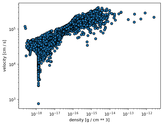
It is thus very common to plot a subset of the cells in scatter plots. Here, we make a scatter plot of density vs temperature, showing only 1 out of 100 cells.

step = 100
osyris.scatter(
    mesh["density"][::step],
    mesh["velocity"][::step],
    loglog=True,
)

<osyris.core.plot.Plot at 0x7bc779270d30>

Coloring the dots

Following Matplotlib’s scatter function signature, the color of the dots can be changed using the color argument:

osyris.scatter(
    mesh["density"][::step], mesh["velocity"][::step], loglog=True, color="red"
)

<osyris.core.plot.Plot at 0x7bc77909b340>

A colormap can also be used to color the dots according to a third quantity, e.g. thermal pressure:

osyris.scatter(
    mesh["density"][::step],
    mesh["velocity"][::step],
    color=mesh["thermal_pressure"][::step],
    norm="log",
    loglog=True,
)

<osyris.core.plot.Plot at 0x7bc7753fb010>

Point size

The size of the dots can be changed using the size parameter. The size can either be a single number:

osyris.scatter(
    mesh["density"][::step],
    mesh["velocity"][::step],
    size=100,
    norm="log",
    loglog=True,
)

<osyris.core.plot.Plot at 0x7bc774d1ca30>

Or it can also be a quantity with physical units

v = mesh["velocity"][::step]

osyris.scatter(v.x, v.y, color="red", size=v * 0.02, aspect="equal")

<osyris.core.plot.Plot at 0x7bc774548070>