Loading Ramses data#
[1]:
import numpy as np
import osyris
Loading a Ramses output#
We load a data output from a star formation simulation
[2]:
path = "osyrisdata/starformation"
data = osyris.RamsesDataset(8, path=path).load()
Processing 12 files in osyrisdata/starformation/output_00008
 16% : read      65623 cells,          0 particles
 25% : read      90140 cells,        956 particles
 33% : read     118232 cells,        956 particles
 41% : read     147100 cells,        956 particles
 50% : read     170244 cells,       2109 particles
 66% : read     235859 cells,       2109 particles
 75% : read     260384 cells,       3065 particles
 83% : read     288476 cells,       3065 particles
 91% : read     312840 cells,       4217 particles
Loaded: 340488 cells, 4218 particles.
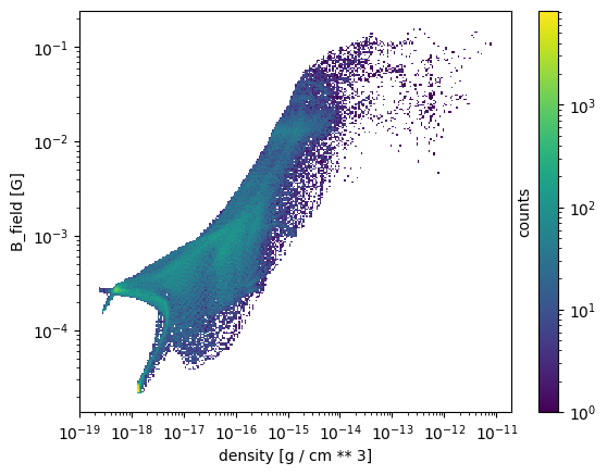
and show a 2D histogram of the gas density versus the magnetic field strength
[3]:
osyris.hist2d(data["mesh"]["density"], data["mesh"]["B_field"], norm="log", loglog=True)
[3]:
<osyris.core.plot.Plot at 0x708bb444d030>
Selective loading#
Filtering on cell values#
It is possible to load only a subset of the cells, by using custom functions to perform the selection.
As an example, to load all the cells with \(\rho > 10^{-15}~{\rm g~cm}^{-3}\), we use a selection criterion
[4]:
data = osyris.RamsesDataset(8, path=path).load(
    select={"mesh": {"density": lambda d: d > 1.0e-15 * osyris.units("g/cm**3")}}
)
Processing 12 files in osyrisdata/starformation/output_00008
 16% : read         23 cells,          0 particles
 25% : read       5064 cells,        956 particles
 33% : read       6550 cells,        956 particles
 41% : read       7635 cells,        956 particles
 50% : read      13259 cells,       2109 particles
 66% : read      13282 cells,       2109 particles
 75% : read      18323 cells,       3065 particles
 83% : read      19809 cells,       3065 particles
 91% : read      23824 cells,       4217 particles
Loaded: 26518 cells, 4218 particles.
and we can now see in the resulting histogram that all the low-density cells have been left out:
[5]:
osyris.hist2d(data["mesh"]["density"], data["mesh"]["B_field"], norm="log", loglog=True)
[5]:
<osyris.core.plot.Plot at 0x708bb1e6af20>

Multiple selection criteria are ANDed:
[6]:
data = osyris.RamsesDataset(8, path=path).load(
    select={
        "mesh": {
            "density": lambda d: d > 1.0e-16 * osyris.units("g/cm**3"),
            "position_x": lambda x: x > 1500.0 * osyris.units("au"),
        },
    }
)
Processing 12 files in osyrisdata/starformation/output_00008
 16% : read       2180 cells,          0 particles
 25% : read      16026 cells,        956 particles
 33% : read      24666 cells,        956 particles
 41% : read      31428 cells,        956 particles
 50% : read      47636 cells,       2109 particles
 66% : read      51327 cells,       2109 particles
 75% : read      65647 cells,       3065 particles
 83% : read      74636 cells,       3065 particles
 91% : read      89198 cells,       4217 particles
Loaded: 99892 cells, 4218 particles.
[7]:
osyris.map(
    data["mesh"].layer("density"),
    dx=1000 * osyris.units("au"),
    origin=data["mesh"]["position"][np.argmax(data["mesh"]["density"])],
    direction="z",
    norm="log",
)
[7]:
<osyris.core.plot.Plot at 0x708baae7bac0>

Only loading certain groups or variables#
It is also possible to select which groups to load. The different groups for the present simulation are mesh, part, and sink. For example, to load only the mesh and sink groups, use
[8]:
data = osyris.RamsesDataset(8, path=path).load(["mesh", "sink"])
data.keys()
Processing 12 files in osyrisdata/starformation/output_00008
 16% : read      65623 cells,          0 particles
 25% : read      90140 cells,          0 particles
 33% : read     118232 cells,          0 particles
 41% : read     147100 cells,          0 particles
 50% : read     170244 cells,          0 particles
 66% : read     235859 cells,          0 particles
 75% : read     260384 cells,          0 particles
 83% : read     288476 cells,          0 particles
 91% : read     312840 cells,          0 particles
Loaded: 340488 cells, 0 particles.
[8]:
dict_keys(['sink', 'mesh'])
It is also possible to load only certain variables in a group by listing them in the same way:
[9]:
data = osyris.RamsesDataset(8, path=path).load(
    select={"mesh": ["density", "position_x", "velocity_y"]}
)
data["mesh"].keys()
Processing 12 files in osyrisdata/starformation/output_00008
 16% : read      65623 cells,          0 particles
 25% : read      90140 cells,        956 particles
 33% : read     118232 cells,        956 particles
 41% : read     147100 cells,        956 particles
 50% : read     170244 cells,       2109 particles
 66% : read     235859 cells,       2109 particles
 75% : read     260384 cells,       3065 particles
 83% : read     288476 cells,       3065 particles
 91% : read     312840 cells,       4217 particles
Loaded: 340488 cells, 4218 particles.
[9]:
dict_keys(['position_x', 'density', 'velocity_y'])
Selecting AMR levels#
Selecting AMR levels uses the same syntax as selecting other variables, but works slightly differently under the hood. A maximum level will be found by testing the selection function provided, and only the required levels will be traversed by the loader, thus speeding up the loading process.
Hence,
[10]:
data = osyris.RamsesDataset(8, path=path).load(
    select={"mesh": {"level": lambda l: l < 7}}
)
data["mesh"]["level"]
Processing 12 files in osyrisdata/starformation/output_00008
 16% : read      29402 cells,          0 particles
 25% : read      29842 cells,        956 particles
 33% : read      43887 cells,        956 particles
 41% : read      48004 cells,        956 particles
 50% : read      53124 cells,       2109 particles
 66% : read      82526 cells,       2109 particles
 75% : read      82966 cells,       3065 particles
 83% : read      97011 cells,       3065 particles
 91% : read      98600 cells,       4217 particles
Loaded: 106248 cells, 4218 particles.
[10]:
'level' Min: 5 Max: 6 [] (106248,)
will only read levels 1 to 6, while
[11]:
data = osyris.RamsesDataset(8, path=path).load(
    select={"mesh": {"level": lambda l: np.logical_and(l > 5, l < 9)}}
)
data["mesh"]["level"]
Processing 12 files in osyrisdata/starformation/output_00008
 16% : read      60265 cells,          0 particles
 25% : read      76654 cells,        956 particles
 33% : read      96290 cells,        956 particles
 41% : read     121166 cells,        956 particles
 50% : read     133758 cells,       2109 particles
 66% : read     194015 cells,       2109 particles
 75% : read     210412 cells,       3065 particles
 83% : read     230904 cells,       3065 particles
 91% : read     247060 cells,       4217 particles
Loaded: 267516 cells, 4218 particles.
[11]:
'level' Min: 6 Max: 8 [] (267516,)
will read levels 1 to 8, but will then discard all cells with level < 6.
Loading only selected CPU outputs#
It is also possible to feed a list of CPU numbers to read from.
[12]:
data = osyris.RamsesDataset(8, path=path).load(cpu_list=[1, 2, 10, 4, 5])
Processing 5 files in osyrisdata/starformation/output_00008
 20% : read      32808 cells,          0 particles
 40% : read      65623 cells,          0 particles
 60% : read      93715 cells,          0 particles
 80% : read     121807 cells,          0 particles
Loaded: 150675 cells, 0 particles.
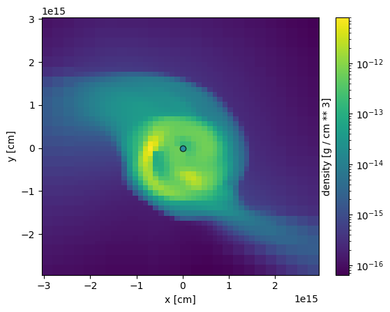
[13]:
osyris.map(
    data["mesh"].layer("density"),
    dx=2000 * osyris.units("au"),
    origin=data["mesh"]["position"][np.argmax(data["mesh"]["density"])],
    direction="z",
    norm="log",
)
[13]:
<osyris.core.plot.Plot at 0x708bab48cee0>
Note
When performing a selection (using select) on spatial position x, y, or z, and if the ordering of the cells in the AMR mesh is using the Hilbert curve, then a pre-selection is automatically made on the CPU files to load to speed-up the loading.
Example: loading a region around a sink particle#
Combining some of the methods illustrated above, we show here how to load only a small region 400 AU wide around a sink particle.
We begin by loading only the sink particle data, by using select=['sink'] in the load method:
[14]:
data = osyris.RamsesDataset(8, path=path).load(select=["sink"])
data
Loaded: 0 cells, 0 particles.
[14]:
Dataset: osyrisdata/starformation/output_00008: 128.00 B

Datagroup: sink 128.00 B
'id' Min: 1.0 Max: 2.0 [] (2,)
'msink' Min: 3.482e+32 Max: 3.485e+32 [g] (2,)
'position' Min: 5.061e+16 Max: 5.192e+16 [cm] (2,), {x,y,z}
'v' Min: 7.464e+04 Max: 7.577e+04 [cm / s] (2,), {x,y,z}
The sink data group contains the positions of the sink particles. We wish to load the region around the first sink particle, which will be the center of our domain.
[15]:
center = data["sink"]["position"][0]
dx = 200 * osyris.units("au")
We are now in a position to load the rest of the data (amr, hydro, etc.) and perform a spatial selection based on the sink’s position (note how the loading below is only looking through 6 files, as opposed to 12 at the top of the notebook, because it uses the knowledge from the Hilbert space-filling curve to skip CPUs that are not connected to the domain of interest).
[16]:
data.load(
    select={
        "mesh": {
            "position_x": lambda x: (x > center.x - dx) & (x < center.x + dx),
            "position_y": lambda y: (y > center.y - dx) & (y < center.y + dx),
            "position_z": lambda z: (z > center.z - dx) & (z < center.z + dx),
        }
    }
)
Processing 6 files in osyrisdata/starformation/output_00008
 16% : read       6816 cells,          0 particles
 33% : read      20520 cells,       1153 particles
 50% : read      20520 cells,       1153 particles
 66% : read      32842 cells,       2109 particles
 83% : read      40543 cells,       2109 particles
Loaded: 40543 cells, 2109 particles.
[16]:
Dataset: osyrisdata/starformation/output_00008: 8.60 MB

Datagroup: sink 128.00 B
'id' Min: 1.0 Max: 2.0 [] (2,)
'msink' Min: 3.482e+32 Max: 3.485e+32 [g] (2,)
'position' Min: 5.061e+16 Max: 5.192e+16 [cm] (2,), {x,y,z}
'v' Min: 7.464e+04 Max: 7.577e+04 [cm / s] (2,), {x,y,z}

Datagroup: mesh 8.43 MB
'level' Min: 8 Max: 9 [] (40543,)
'cpu' Min: 3 Max: 6 [] (40543,)
'dx' Min: 1.151e+14 Max: 2.303e+14 [cm] (40543,)
'density' Min: 4.702e-17 Max: 8.047e-12 [g / cm ** 3] (40543,)
'thermal_pressure' Min: 1.703e-08 Max: 0.057 [erg / cm ** 3] (40543,)
'internal_energy' Min: 2.555e-08 Max: 0.085 [erg / cm ** 3] (40543,)
'temperature' Min: 10.060 Max: 196.393 [K] (40543,)
'grav_potential' Min: -6.219e+12 Max: -5.543e+11 [cm ** 2 / s ** 2] (40543,)
'position' Min: 4.569e+16 Max: 5.561e+16 [cm] (40543,), {x,y,z}
'velocity' Min: 1.024e+04 Max: 4.216e+05 [cm / s] (40543,), {x,y,z}
'B_left' Min: 1.174e-04 Max: 0.162 [G] (40543,), {x,y,z}
'B_right' Min: 1.155e-04 Max: 0.162 [G] (40543,), {x,y,z}
'grav_acceleration' Min: 2.263e-06 Max: 2.028e-04 [cm / s ** 2] (40543,), {x,y,z}
'B_field' Min: 1.197e-04 Max: 0.157 [G] (40543,), {x,y,z}
'mass' Min: 6.851e-08 Max: 0.006 [M_sun] (40543,)

Datagroup: part 168.72 KB
'mass' Min: 1.652e+29 Max: 1.652e+29 [g] (2109,)
'identity' Min: -1.0 Max: -1.0 [] (2109,)
'levelp' Min: 5.0 Max: 5.0 [] (2109,)
'birth_time' Min: 8.888e-05 Max: 8.888e-05 [] (2109,)
'position' Min: 5.017e+16 Max: 5.105e+16 [cm] (2109,), {x,y,z}
'velocity' Min: 7.464e+04 Max: 7.464e+04 [cm / s] (2109,), {x,y,z}
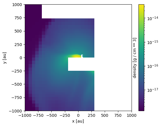
Finally, we can make a map of the gas density around our sink particle (note that no spatial limits are specified in the map call, it is making a map using all the cells that have been loaded)
[17]:
osyris.map(
    data["mesh"].layer("density"),
    data["sink"].layer(
        "position",
        mode="scatter",
        c="white",
        s=20.0 * osyris.units("au"),
        alpha=0.7,
    ),
    norm="log",
    direction="z",
    origin=center,
)
[17]:
<osyris.core.plot.Plot at 0x708bab29feb0>