Basics

This notebook provides a quick introduction on how to get started with loading a simulation output and creating some basic figures.

The data files used in these documentation pages can be found here.

Reading a RAMSES output

Import the osyris module and load the output of your choice. We are loading output number 8 from a simulation of a collapsing system of gas, that is forming young stars in its core.

IMPORTANT

The data loader searches for descriptor files (hydro_file_descriptor.txt, rt_file_descriptor and the like) inside the output directory to get the variable names.

If your version of RAMSES does not support this (the file descriptor did not exist in old versions of RAMSES), you will need to generate one and copy it into each of your output directories.

import osyris
import numpy as np

data = osyris.RamsesDataset(8, path="osyrisdata/starformation")

When creating a RamsesDataset, the first argument is the output number. Note that you can use -1 to select the last output in the directory.

Upon creation, the Dataset only reads the simulation metadata, and does not load the bulk of the simulation data.

To actually load the data, we call the load() method on the Dataset. The Dataset has a __str__ representation, which will return a list of all the variables contained in the loaded file, along with their minimum and maximum values.

data.load()

Processing 12 files in osyrisdata/starformation/output_00008
 16% : read      65623 cells,          0 particles
 25% : read      90140 cells,        956 particles
 33% : read     118232 cells,        956 particles
 41% : read     147100 cells,        956 particles
 50% : read     170244 cells,       2109 particles
 66% : read     235859 cells,       2109 particles
 75% : read     260384 cells,       3065 particles
 83% : read     288476 cells,       3065 particles
 91% : read     312840 cells,       4217 particles
Loaded: 340488 cells, 4218 particles.

Dataset: osyrisdata/starformation/output_00008: 71.16 MB

Datagroup: sink 128.00 B
'id' Min: 1.0 Max: 2.0 [] (2,)
'msink' Min: 3.482e+32 Max: 3.485e+32 [g] (2,)
'position' Min: 5.061e+16 Max: 5.192e+16 [cm] (2,), {x,y,z}
'v' Min: 7.464e+04 Max: 7.577e+04 [cm / s] (2,), {x,y,z}

Datagroup: mesh 70.82 MB
'level' Min: 5 Max: 9 [] (340488,)
'cpu' Min: 1 Max: 12 [] (340488,)
'dx' Min: 1.151e+14 Max: 1.842e+15 [cm] (340488,)
'density' Min: 2.376e-19 Max: 8.047e-12 [g / cm ** 3] (340488,)
'thermal_pressure' Min: 8.555e-11 Max: 0.057 [erg / cm ** 3] (340488,)
'internal_energy' Min: 1.283e-10 Max: 0.085 [erg / cm ** 3] (340488,)
'temperature' Min: 10.002 Max: 196.393 [K] (340488,)
'grav_potential' Min: -6.219e+12 Max: 9.126e+10 [cm ** 2 / s ** 2] (340488,)
'position' Min: 1.595e+15 Max: 1.005e+17 [cm] (340488,), {x,y,z}
'velocity' Min: 742.189 Max: 4.216e+05 [cm / s] (340488,), {x,y,z}
'B_left' Min: 2.097e-05 Max: 0.164 [G] (340488,), {x,y,z}
'B_right' Min: 2.097e-05 Max: 0.162 [G] (340488,), {x,y,z}
'grav_acceleration' Min: 4.196e-09 Max: 2.028e-04 [cm / s ** 2] (340488,), {x,y,z}
'B_field' Min: 2.119e-05 Max: 0.157 [G] (340488,), {x,y,z}
'mass' Min: 5.721e-08 Max: 0.006 [M_sun] (340488,)

Datagroup: part 337.44 KB
'mass' Min: 1.651e+29 Max: 1.652e+29 [g] (4218,)
'identity' Min: -2.0 Max: -1.0 [] (4218,)
'levelp' Min: 5.0 Max: 5.0 [] (4218,)
'birth_time' Min: 8.888e-05 Max: 8.892e-05 [] (4218,)
'position' Min: 5.017e+16 Max: 5.237e+16 [cm] (4218,), {x,y,z}
'velocity' Min: 7.464e+04 Max: 7.577e+04 [cm / s] (4218,), {x,y,z}

The Dataset behaves very much like a Python dictionary. The data it contains is divided into Datagroups, which can be accessed just like accessing elements of a dictionary.

data.keys()

dict_keys(['sink', 'mesh', 'part'])

To access a single variable array, we access entries in a Datagroup in the same way:

data["mesh"]["density"]

'density' Min: 2.376e-19 Max: 8.047e-12 [g / cm ** 3] (340488,)

The information printed is the name of the variable, its minimum and maximum value, its physical unit, and the number of elements (or cells) in the array.

Creating a 2D histogram

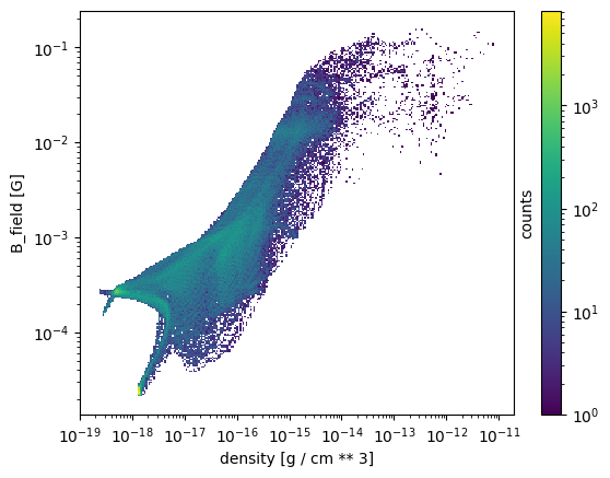
We now wish to plot a 2d histogram of the logarithm of density versus logarithm of magnetic field magnitude, for all the cells inside the computational domain. We also use a logarithmic colormap which represents the cell counts in the \((\rho,B)\) plane

osyris.hist2d(data["mesh"]["density"], data["mesh"]["B_field"], norm="log", loglog=True)

<osyris.core.plot.Plot at 0x7e3769c4a890>

Simple 2D map

The goal here is to create a 2D gas density slice, 2000 au wide, through the plane normal to z, that passes through the center of the young star forming system.

We first need to define where the center of the system is. A simple definition is to use the coordinate of the cell with the highest density in the simulation.

mesh = data["mesh"]
ind = np.argmax(mesh["density"])
center = mesh["position"][ind]
center

'position' Value: 2.470e+16, 3.241e+16, 2.942e+16 [cm] (), {x,y,z}

Once we have this center coordinate, we can use it as the origin for our cut plane and create a map:

osyris.map(
    mesh.layer("density"),
    dx=2000 * osyris.units("au"),
    norm="log",
    origin=center,
    direction="z",
)

<osyris.core.plot.Plot at 0x7e3764879810>

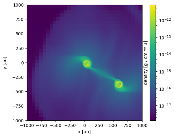
where the first argument is the variable to display, dx is the extent of the viewing region, and direction is the normal to the slicing plane.