Plotting: particles

In this notebook, we will load a cosmological simulation and visualize the dark matter particles within it.

A basic look at the particle positions

import osyris

path = "osyrisdata/cosmology"
data = osyris.RamsesDataset(100, path=path).load("part")

Processing 12 files in osyrisdata/cosmology/output_00100
 16% : read          0 cells,      51942 particles
 25% : read          0 cells,      67911 particles
 33% : read          0 cells,      93994 particles
 41% : read          0 cells,     118197 particles
 50% : read          0 cells,     140830 particles
 66% : read          0 cells,     183389 particles
 75% : read          0 cells,     203902 particles
 83% : read          0 cells,     219136 particles
 91% : read          0 cells,     240981 particles
Loaded: 0 cells, 262144 particles.

We convert the particle masses to solar masses, and their positions to megaparsecs:

part = data["part"]

part["mass"] = part["mass"].to("M_sun")
part["position"] = part["position"].to("Mpc")
part

Datagroup: part 23.07 MB
'mass' Min: 4.159e+11 Max: 4.159e+11 [M_sun] (262144,)
'identity' Min: 1.0 Max: 2.621e+05 [] (262144,)
'levelp' Min: 6.0 Max: 11.0 [] (262144,)
'family' Min: 1.0 Max: 1.0 [] (262144,)
'tag' Min: 0.0 Max: 0.0 [] (262144,)
'position' Min: 3.297 Max: 247.112 [Mpc] (262144,), {x,y,z}
'velocity' Min: 2.854e+05 Max: 2.678e+08 [cm / s] (262144,), {x,y,z}

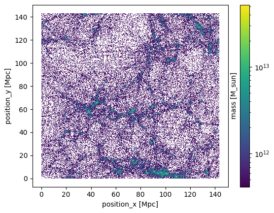
Having loaded the particle data, we can quickly inspect the distribution of the particles by histogramming their x and y positions. We use the particle mass as weights for the histogramming, to give us a feel for how much mass is contained in one of the pixels of the image below.

osyris.hist2d(
    part["position"].x,
    part["position"].y,
    part["mass"],
    bins=512,
    norm="log",
)

<osyris.core.plot.Plot at 0x7fb6ad8e9f30>

Sorting particles

When particles are loaded, they are read in in the order they are stored on disk. It can however often be useful to sort particles according to one of the keys. A common choice is to sort them according to their identity using the .sortby() method of the Datagroup.

print(part["identity"][:20].values)
part.sortby("identity")
print(part["identity"][:20].values)

[ 2.  5. 10. 12. 15. 20. 24. 25. 27. 28. 29. 30. 32. 34. 37. 42. 46. 47.
 52. 54.]
[ 1.  2.  3.  4.  5.  6.  7.  8.  9. 10. 11. 12. 13. 14. 15. 16. 17. 18.
 19. 20.]

It is also possible to apply sorting by using a keyword argument in the load() function:

data = osyris.RamsesDataset(100, path=path).load("part", sortby={"part": "identity"})
print(data["part"]["identity"][:20].values)

Processing 12 files in osyrisdata/cosmology/output_00100
 16% : read          0 cells,      51942 particles
 25% : read          0 cells,      67911 particles
 33% : read          0 cells,      93994 particles
 41% : read          0 cells,     118197 particles
 50% : read          0 cells,     140830 particles
 66% : read          0 cells,     183389 particles
 75% : read          0 cells,     203902 particles
 83% : read          0 cells,     219136 particles
 91% : read          0 cells,     240981 particles
Loaded: 0 cells, 262144 particles.
[ 1.  2.  3.  4.  5.  6.  7.  8.  9. 10. 11. 12. 13. 14. 15. 16. 17. 18.
 19. 20.]

3D rendering

Osyris does not support 3D plotting out of the box, but a 3D rendering of the particle positions in space can be achieved relatively easily in a Jupyter notebook using the pythreejs library (or any other library with 3D capabilities).

Note

pythreejs is not a hard-dependency of Osyris. It needs to be installed separatey with pip install pythreejs.

import pythreejs as p3
import numpy as np

# Only plot one in 10 points to reduce the size of the output
pos = part["position"][::10]
pos_array = np.array([pos.x.values, pos.y.values, pos.z.values]).T.astype("float32")

# Create a position buffer geometry
geometry = p3.BufferGeometry(
    attributes={"position": p3.BufferAttribute(array=pos_array - 75)}
)
# Create a points material
material = p3.PointsMaterial(color="black", size=1)
# Combine the geometry and material into a Points object
points = p3.Points(geometry=geometry, material=material)

# Create the scene and the renderer
view_width = 700
view_height = 500
camera = p3.PerspectiveCamera(position=[200.0, 0, 0], aspect=view_width / view_height)
scene = p3.Scene(children=[points, camera], background="#DDDDDD")
controller = p3.OrbitControls(controlling=camera)
renderer = p3.Renderer(
    camera=camera,
    scene=scene,
    controls=[controller],
    width=view_width,
    height=view_height,
)
renderer