Custom datasets

In the previous notebook, we showed how to load data from a Ramses simulation.

This notebook will show how to create a Datagroup from scratch, using Numpy arrays. This is useful if you want to load data created by a program other than Ramses, for example.

import numpy as np
import osyris
from osyris import Array, Vector

Generate Arrays and Vector from random points

The minimal data needed by osyris to be able to create most plots is:

• position: positions in space

• dx: cell size (the edge of a cube that represents a mesh cell)

• any scalar or vector value (we will make a density here)

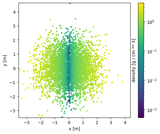
We create x, y, and z positions using ramdon values with a normal distribution, and a unique size for all cells. We also create some fake density values, that correlate to the absolute value of the x position.

N = 100_000
x = Array(values=np.random.normal(size=N), unit="m")
y = Array(values=np.random.normal(size=N), unit="m")
z = Array(values=np.random.normal(size=N), unit="m")

dx = Array(values=np.full(N, 0.1), unit="m")

density = Array(values=np.abs(x.values), unit="g/cm^3")

pos = Vector(x, y, z)

We now populate a Datagroup with all 3:

dg = osyris.Datagroup(position=pos, dx=dx, density=density)
dg

Datagroup:  4.00 MB
'position' Min: 0.016 Max: 5.047 [m] (100000,), {x,y,z}
'dx' Min: 0.1 Max: 0.1 [m] (100000,)
'density' Min: 8.903e-06 Max: 4.330 [g / cm ** 3] (100000,)

Visualization

We can now visualize the data.

Plotting a map

To plot a map of the particle densities, use

osyris.map(dg.layer("density"), norm="log", direction="z")

<osyris.core.plot.Plot at 0x75619208a1a0>

Plotting a histogram

A one-dimensional histogram is obtained with

osyris.hist1d(dg["density"])

<osyris.core.plot.Plot at 0x7561a7f74f10>

The rest of the documentation focuses on all the different plotting methods that are available.